dream analysis
Differential expression testing with linear mixed models for repeated measures
Developed by Gabriel Hoffman
Run on 2026-03-19 09:16:57
Source:vignettes/dream.Rmd
dream.RmdDifferential expression for repeated measures (dream) uses a linear model model to increase power and decrease false positives for RNA-seq datasets with multiple measurements per individual. The analysis fits seamlessly into the widely used workflow of limma/voom (Law et al. 2014). Dream uses a linear model model to increase power and decrease false positives for RNA-seq datasets with repeated measurements. Dream achieves this by combining multiple statistical concepts into a single statistical model. The model includes:
- flexible modeling of repeated measures gene expression data
- precision weights to model measurement error in RNA-seq
counts
- ability to model multiple random effects
- random effects estimated separately for each gene
- hypothesis testing for fixed effects in linear mixed models
- small sample size hypothesis test
Dream also includes multi-threaded analysis across thousands of genes on a multi-core machine.
Standard RNA-seq processing
This tutorial assumes that the reader is familiar with the limma/voom workflow for RNA-seq. Process raw count data using limma/voom.
library("variancePartition")
library("edgeR")
library("BiocParallel")
data(varPartDEdata)

# filter genes by number of counts
isexpr <- rowSums(cpm(countMatrix) > 0.1) >= 5

# Standard usage of limma/voom
dge <- DGEList(countMatrix[isexpr, ])
dge <- calcNormFactors(dge)

# make this vignette faster by analyzing a subset of genes
dge <- dge[1:1000, ]
Limma Analysis
Limma has a built-in approach for analyzing repeated measures data
using duplicateCorrelation(). The model can handle a single
random effect, and forces the magnitude of the random effect to be the
same across all genes.
# apply duplicateCorrelation is two rounds
design <- model.matrix(~Disease, metadata)
vobj_tmp <- voom(dge, design, plot = FALSE)
dupcor <- duplicateCorrelation(vobj_tmp, design, block = metadata$Individual)

# run voom considering the duplicateCorrelation results
# in order to compute more accurate precision weights
# Otherwise, use the results from the first voom run
vobj <- voom(dge, design, plot = FALSE, block = metadata$Individual, correlation = dupcor$consensus)

# Estimate linear mixed model with a single variance component
# Fit the model for each gene,
dupcor <- duplicateCorrelation(vobj, design, block = metadata$Individual)

# But this step uses only the genome-wide average for the random effect
fitDupCor <- lmFit(vobj, design, block = metadata$Individual, correlation = dupcor$consensus)

# Fit Empirical Bayes for moderated t-statistics
fitDupCor <- eBayes(fitDupCor)
Dream Analysis
The dream method replaces 4 core functions of limma with a linear mixed model.
-
voomWithDreamWeights()replacesvoom()to estimate precision weights -
dream()replaceslmFit()to estimate regression coefficients.
-
variancePartition::eBayes()replaceslimma::eBayes()to apply empircal Bayes shrinkage on linear mixed models. -
variancePartition::topTable()replaceslimma::topTable()to give seamless access to results fromdream().
For models with only fixed effects,
variancePartition::eBayes(), and
variancePartition::topTable() work seamlessly and give
results equivalent to the limma functions with the same
name. From the user perspective, the dream() workflow is
the same as limma since the statistical differences are
handled behind the scenes.
# Specify parallel processing parameters
# this is used implicitly by dream() to run in parallel
param <- SnowParam(4, "SOCK", progressbar = TRUE)

# The variable to be tested must be a fixed effect
form <- ~ Disease + (1 | Individual)

# estimate weights using linear mixed model of dream
vobjDream <- voomWithDreamWeights(dge, form, metadata, BPPARAM = param)

# Fit the dream model on each gene
# For the hypothesis testing, by default,
# dream() uses the KR method for <= 20 samples,
# otherwise it uses the Satterthwaite approximation
fitmm <- dream(vobjDream, form, metadata)
fitmm <- eBayes(fitmm)
# Examine design matrix
head(fitmm$design, 3)
## (Intercept) Disease1
## sample_01 1 0
## sample_02 1 0
## sample_03 1 0
# Get results of hypothesis test on coefficients of interest
topTable(fitmm, coef = "Disease1", number = 3)
## logFC AveExpr t P.Value adj.P.Val B
## ENST00000283033.5 gene=TXNDC11 1.556233 3.567624 32.18311 2.963157e-21 2.963157e-18 38.37597
## ENST00000257181.9 gene=PRPF38A 1.380549 4.398270 24.31101 2.046048e-18 1.023024e-15 32.17816
## ENST00000525790.1 gene=TDRKH 1.508341 3.184931 19.20262 4.498201e-16 1.261794e-13 26.87813
## z.std
## ENST00000283033.5 gene=TXNDC11 9.464024
## ENST00000257181.9 gene=PRPF38A 8.754723
## ENST00000525790.1 gene=TDRKH 8.124335Since dream uses an estimated degrees of freedom value for each
hypothsis test, the degrees of freedom is different for each gene here.
Therefore, the t-statistics are not directly comparable since they have
different degrees of freedom. In order to be able to compare test
statistics, we report z.std which is the p-value
transformed into a signed z-score. This can be used for downstream
analysis.
Note that if a random effect is not specified, dream()
automatically uses lmFit(), but the user must run
eBayes() afterward.
Advanced hypothesis testing
Using contrasts to compare coefficients
You can also perform a hypothesis test of the difference
between two or more coefficients by using a contrast matrix. The
contrasts are evaluated at the time of the model fit and the results can
be extracted with topTable(). This behaves like
makeContrasts() and contrasts.fit() in
limma.
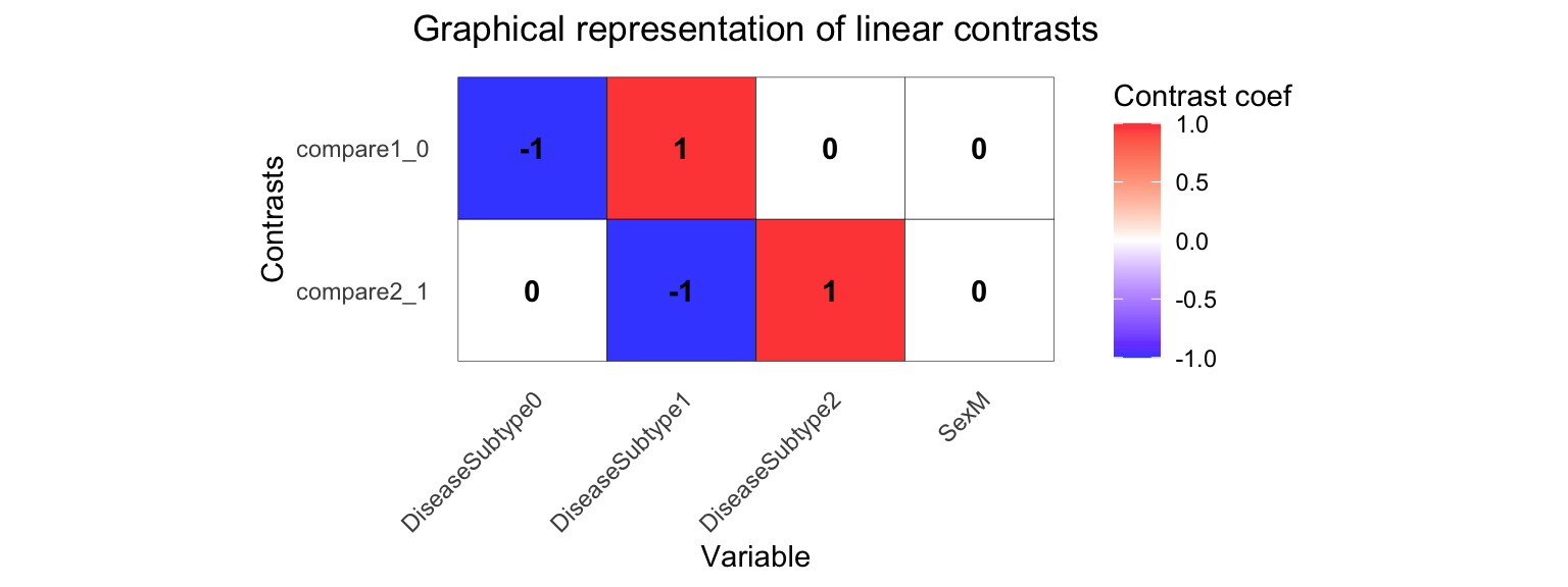
Multiple contrasts can be evaluated at the same time, in order to save computation time. Make sure to inspect your contrast matrix to confirm it is testing what you intend.
form <- ~ 0 + DiseaseSubtype + Sex + (1 | Individual)

L <- makeContrastsDream(form, metadata,
  contrasts = c(
    compare2_1 = "DiseaseSubtype2 - DiseaseSubtype1",
    compare1_0 = "DiseaseSubtype1 - DiseaseSubtype0"
  )
)

# Visualize contrast matrix
plotContrasts(L)
# fit dream model with contrasts
fit <- dream(vobjDream, form, metadata, L)
fit <- eBayes(fit)

# get names of available coefficients and contrasts for testing
colnames(fit)
## [1] "compare2_1" "compare1_0" "DiseaseSubtype0" "DiseaseSubtype1" "DiseaseSubtype2"
## [6] "SexM"
# extract results from first contrast
topTable(fit, coef = "compare2_1", number = 3)
## logFC AveExpr t P.Value adj.P.Val B
## ENST00000355624.3 gene=RAB11FIP2 -0.9493146 5.260280 -5.336063 2.343973e-05 0.02343973 0.8221724
## ENST00000593466.1 gene=DDA1 -1.7265710 3.901579 -3.659542 1.378483e-03 0.68924129 -1.5680931
## ENST00000200676.3 gene=CETP 1.4777422 3.723438 3.865319 4.126594e-03 0.99948768 -1.8592924
## z.std
## ENST00000355624.3 gene=RAB11FIP2 -4.229321
## ENST00000593466.1 gene=DDA1 -3.199119
## ENST00000200676.3 gene=CETP 2.868319Comparing multiple coefficients
So far contrasts have only involved the difference between two
coefficients. But contrasts can also compare any linear combination of
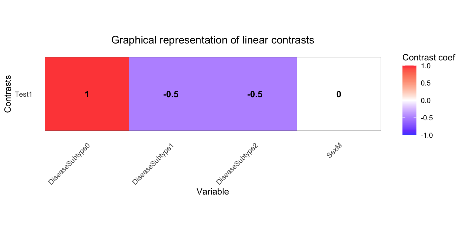
coefficients. Here, consider comparing DiseaseSubtype0 to
the mean of DiseaseSubtype1 and
DiseaseSubtype2. Note you can also customize the name of
the contrast.
L2 <- makeContrastsDream(form, metadata,
  contrasts =
    c(Test1 = "DiseaseSubtype0 - (DiseaseSubtype1 + DiseaseSubtype2)/2")
)

plotContrasts(L2)
# fit dream model to evaluate contrasts
fit <- dream(vobjDream[1:10, ], form, metadata, L = L2)
fit <- eBayes(fit)

topTable(fit, coef = "Test1", number = 3)
## logFC AveExpr t P.Value adj.P.Val B
## ENST00000418210.2 gene=TMEM64 -1.0343236 4.715367 -6.874897 2.770467e-07 2.770467e-06 8.410269
## ENST00000456159.1 gene=MET -0.9830788 2.458926 -6.021668 5.553855e-07 2.776928e-06 5.915610
## ENST00000555834.1 gene=RPS6KL1 -0.8954795 5.272063 -5.419044 3.684288e-06 1.228096e-05 4.056947
## z.std
## ENST00000418210.2 gene=TMEM64 -5.138428
## ENST00000456159.1 gene=MET -5.006119
## ENST00000555834.1 gene=RPS6KL1 -4.628441Joint hypothesis test of multiple coefficients
Joint hypothesis testing of multiple coefficients at the same time
can be performed by using an F-test. Just like in limma, the results can
be extracted using topTable()
# extract results from first contrast
topTable(fit, coef = c("DiseaseSubtype2", "DiseaseSubtype1"), number = 3)
## DiseaseSubtype2 DiseaseSubtype1 AveExpr F P.Value
## ENST00000418210.2 gene=TMEM64 5.301001 5.211674 4.715367 794.2599 2.087246e-24
## ENST00000555834.1 gene=RPS6KL1 5.662699 5.719196 5.272063 782.3692 2.541435e-24
## ENST00000589123.1 gene=NFIC 6.545195 6.181023 5.855335 659.9594 2.333522e-23
## adj.P.Val F.std
## ENST00000418210.2 gene=TMEM64 1.270717e-23 54.52620
## ENST00000555834.1 gene=RPS6KL1 1.270717e-23 54.32931
## ENST00000589123.1 gene=NFIC 7.778406e-23 52.11208Since dream uses an estimated degrees of freedom value for each
hypothsis test, the degrees of freedom is different for each gene here.
Therefore, the F-statistics are not directly comparable since they have
different degrees of freedom. In order to be able to compare test
statistics, we report F.std which is the p-value
transformed into an F-statistic with df_1 the number of coefficients tested and
df_2=\infty. This can be used for
downstream analysis.
Small-sample method
For small datasets, the Kenward-Roger method can be more powerful. But it is substantially more computationally intensive.
variancePartition plot
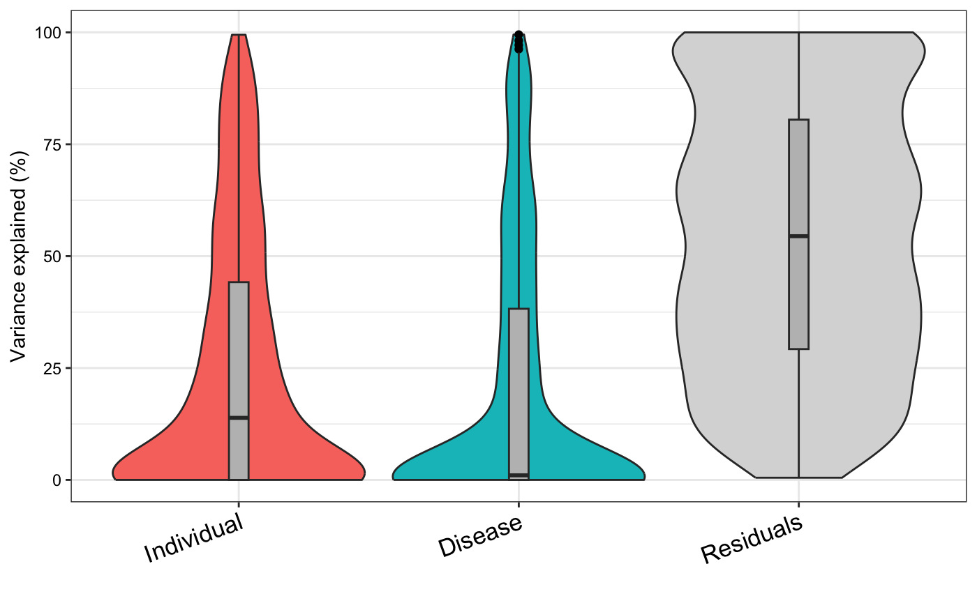
Dream and variancePartition share the same underlying linear mixed model framework. A variancePartition analysis can indicate important variables that should be included as fixed or random effects in the dream analysis.
# Note: this could be run with either vobj from voom()
# or vobjDream from voomWithDreamWeights()
# The resuylts are similar
form <- ~ (1 | Individual) + (1 | Disease)
vp <- fitExtractVarPartModel(vobj, form, metadata)

plotVarPart(sortCols(vp))
Comparing p-values
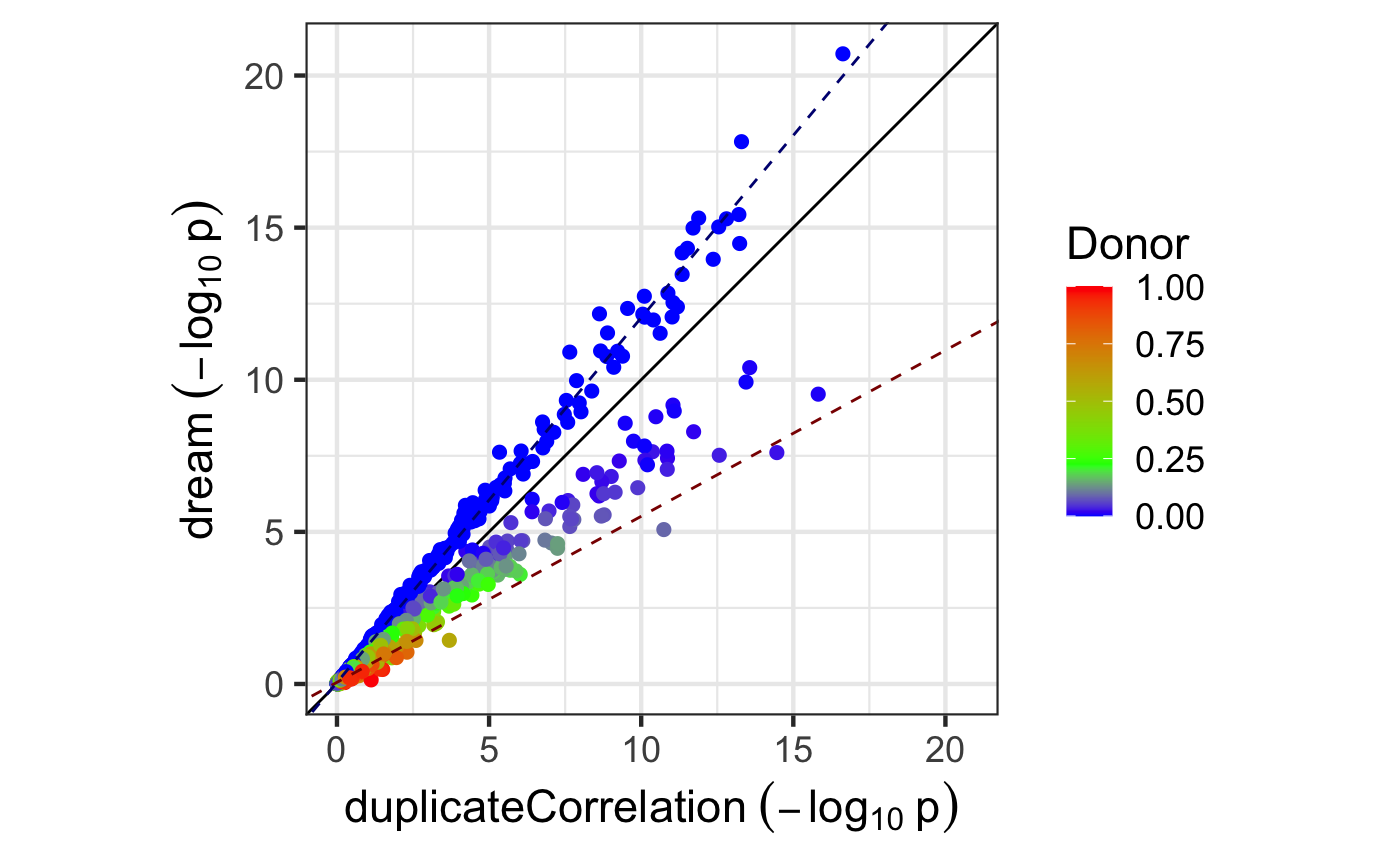
Here we compare p-values from from dream() and
duplicateCorrelation. In order to understand the empircal
difference between them, we can plot the -\log_{10} p-values from each method.
# Compare p-values and make plot
p1 <- topTable(fitDupCor, coef = "Disease1", number = Inf, sort.by = "none")$P.Value
p2 <- topTable(fitmm, number = Inf, sort.by = "none")$P.Value

plotCompareP(p1, p2, vp$Individual, dupcor$consensus)
The duplicateCorrelation method estimates a single variance term genome-wide even though the donor contribution of a particular gene can vary substantially from the genome-wide trend. Using a single value genome-wide for the within-donor variance can reduce power and increase the false positive rate in a particular, reproducible way. Let \tau^2_g be the value of the donor component for gene g and \bar{\tau}^2 be the genome-wide mean. For genes where \tau^2_g>\bar{\tau}^2, using \bar{\tau}^2 under-corrects for the donor component so that it increases the false positive rate compared to using \tau^2_g. Conversely, for genes where \tau^2_g<\bar{\tau}^2, using \bar{\tau}^2 over-corrects for the donor component so that it decreases power. Increasing sample size does not overcome this issue. The dream method overcomes this issue by using a \tau^2_g.
Here, the -\log_{10} p-values from both methods are plotted and colored by the donor contribution estiamted by variancePartition. The green value indicates \bar{\tau}^2, while red and blue indicate higher and lower values, respectively. When only one variance component is used and the contrast matrix is simple, the effect of using dream versus duplicateCorrelation is determined by the comparison of \tau^2_g to \bar{\tau}^2:
dream can increase the -\log_{10} p-value for genes with a lower donor component (i.e. \tau^2_g<\bar{\tau}^2) and decrease -\log_{10} p-value for genes with a higher donor component (i.e. \tau^2_g>\bar{\tau}^2)
Note that using more variance components or a more complicated contrast matrix can make the relationship more complicated.
Parallel processing
variancePartition functions including dream(),
fitExtractVarPartModel() and fitVarPartModel()
can take advange of multicore machines to speed up analysis. It uses the
BiocParallel
package to manage the parallelization.
- Specify parameters with the BPPARAM argument.
# Request 4 cores, and enable the progress bar
# This is the ideal for Linux, OS X and Windows
param <- SnowParam(4, "SOCK", progressbar = TRUE)
fitmm <- dream(vobjDream, form, metadata, BPPARAM = param)
By default BPPARAM = SerialParam().
Session info
## R version 4.5.1 (2025-06-13)
## Platform: aarch64-apple-darwin23.6.0
## Running under: macOS Sonoma 14.7.1
##
## Matrix products: default
## BLAS/LAPACK: /opt/homebrew/Cellar/openblas/0.3.30/lib/libopenblasp-r0.3.30.dylib;  LAPACK version 3.12.0
##
## locale:
## [1] en_US.UTF-8/en_US.UTF-8/en_US.UTF-8/C/en_US.UTF-8/en_US.UTF-8
##
## time zone: America/New_York
## tzcode source: internal
##
## attached base packages:
## [1] stats     graphics  grDevices utils     datasets  methods   base
##
## other attached packages:
## [1] edgeR_4.6.3              variancePartition_1.39.5 BiocParallel_1.42.2
## [4] limma_3.64.3             ggplot2_4.0.1            pander_0.6.6
##
## loaded via a namespace (and not attached):
##  [1] tidyselect_1.2.1    dplyr_1.1.4         farver_2.1.2        S7_0.2.1
##  [5] bitops_1.0-9        fastmap_1.2.0       digest_0.6.39       lifecycle_1.0.4
##  [9] statmod_1.5.1       magrittr_2.0.4      compiler_4.5.1      rlang_1.1.6
## [13] sass_0.4.10         tools_4.5.1         yaml_2.3.10         knitr_1.50
## [17] labeling_0.4.3      htmlwidgets_1.6.4   plyr_1.8.9          RColorBrewer_1.1-3
## [21] KernSmooth_2.23-26  withr_3.0.2         purrr_1.2.0         numDeriv_2016.8-1.1
## [25] BiocGenerics_0.54.1 desc_1.4.3          grid_4.5.1          aod_1.3.3
## [29] caTools_1.18.3      scales_1.4.0        gtools_3.9.5        iterators_1.0.14
## [33] MASS_7.3-65         dichromat_2.0-0.1   cli_3.6.5           mvtnorm_1.3-3
## [37] rmarkdown_2.30      ragg_1.5.0          reformulas_0.4.2    generics_0.1.4
## [41] reshape2_1.4.5      minqa_1.2.8         cachem_1.1.0        stringr_1.6.0
## [45] splines_4.5.1       parallel_4.5.1      matrixStats_1.5.0   vctrs_0.6.5
## [49] boot_1.3-32         Matrix_1.7-4        jsonlite_2.0.0      pbkrtest_0.5.5
## [53] systemfonts_1.3.1   locfit_1.5-9.12     jquerylib_0.1.4     tidyr_1.3.1
## [57] snow_0.4-4          glue_1.8.0          pkgdown_2.2.0       nloptr_2.2.1
## [61] codetools_0.2-20    stringi_1.8.7       gtable_0.3.6        EnvStats_3.1.0
## [65] lme4_1.1-38         lmerTest_3.1-3      tibble_3.3.0        remaCor_0.0.20
## [69] pillar_1.11.1       htmltools_0.5.8.1   gplots_3.2.0        R6_2.6.1
## [73] textshaping_1.0.4   Rdpack_2.6.4        evaluate_1.0.5      lattice_0.22-7
## [77] Biobase_2.68.0      rbibutils_2.4       backports_1.5.0     RhpcBLASctl_0.23-42
## [81] broom_1.0.10        fANCOVA_0.6-1       corpcor_1.6.10      bslib_0.9.0
## [85] Rcpp_1.1.0          nlme_3.1-168        xfun_0.54           fs_1.6.6
## [89] pkgconfig_2.0.3
<>