Normal approximation vs. empirical simulation

Asymptotic normal approximation

Let the vector \({\bf p}\) be the true fractions across \(D\) categories. Consider \(C\) total counts sampled from a Dirichlet-multinomial (DMN) distribution with overdispersion \(\tau\), where \(\tau=1\) reduces to the multinomial distribution. The centered log ratio (CLR) of the \(i^{th}\) estimated fraction in \({\bf \hat p}\) is

\[\begin{equation} \tag{1} \text{clr}_i({\bf \hat p}) = \log(\hat p_i) - \frac{1}{D}\sum_{j=1}^D \log(\hat p_j) \end{equation}\] and we show that the sampling variance is

\[\begin{equation} \tag{2} \text{var}[\text{clr}_i({\bf \hat p})] = \frac{\tau}{C} \left[ \frac{1}{\hat p_i} - \frac{2}{ D \hat p_i} + \frac{1}{D^2}\sum_{j=1}^D \frac{1}{\hat p_j} \right]. \label{eqn2} \end{equation}\]

Simulations

The sampling variance is derived from asymototic theory, so we examine its behavior for finite total counts. Here we evalute the emprical variance from \(1,000\) draws from a Dirichlet-multinomial distribution while varying \(D\), \(\tau\), \(C\). A pseudocount of 0.5 is added to the observed counts since the asymptotic theory is not defined for counts of zero.

Here we plot the standard deviation after CLR transform from the empirical DMN and the asymptotic normal approximation under a range of conditions. Results are shown for instances with at least 2 counts.

D=2 categories

D=15 categories

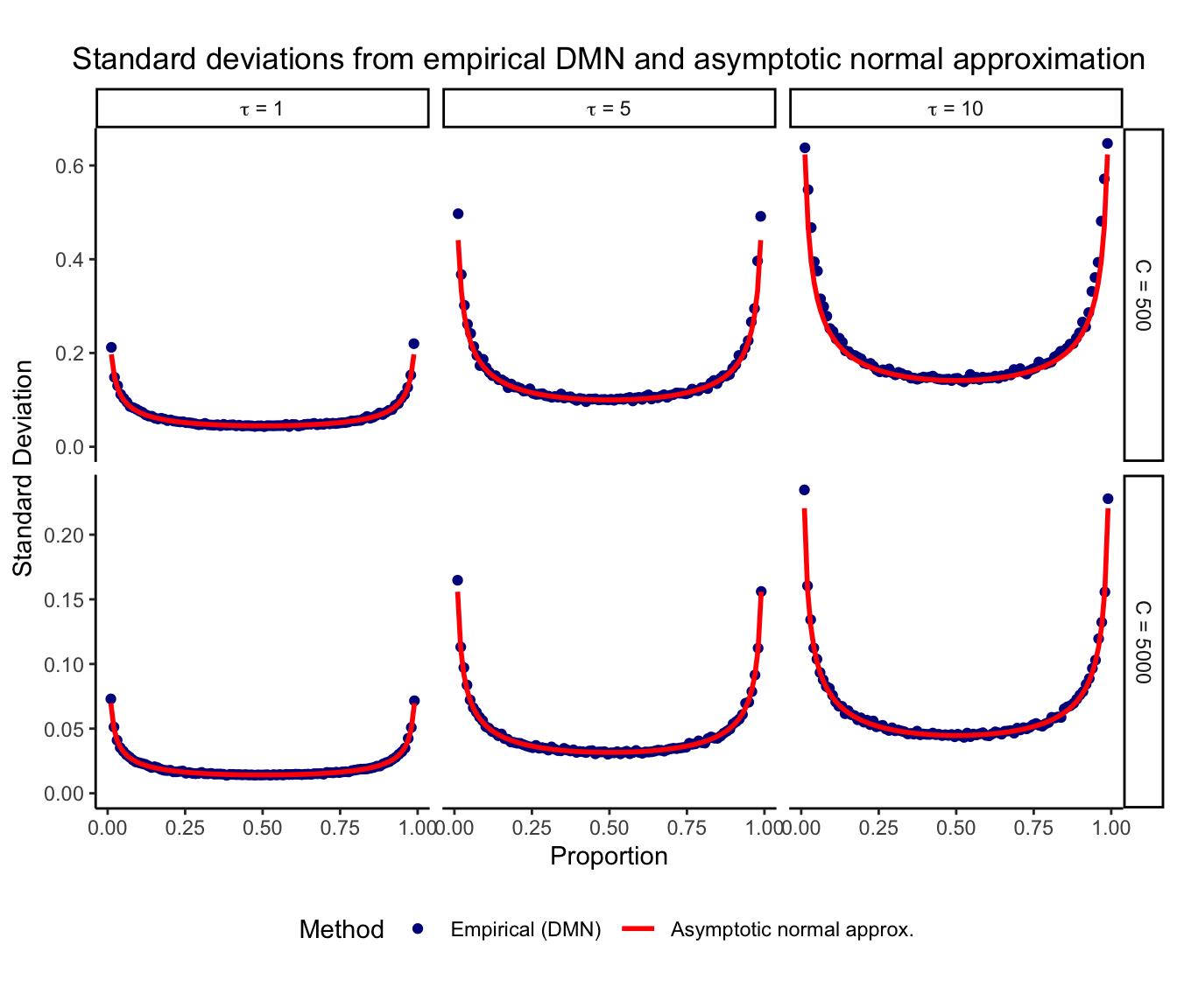
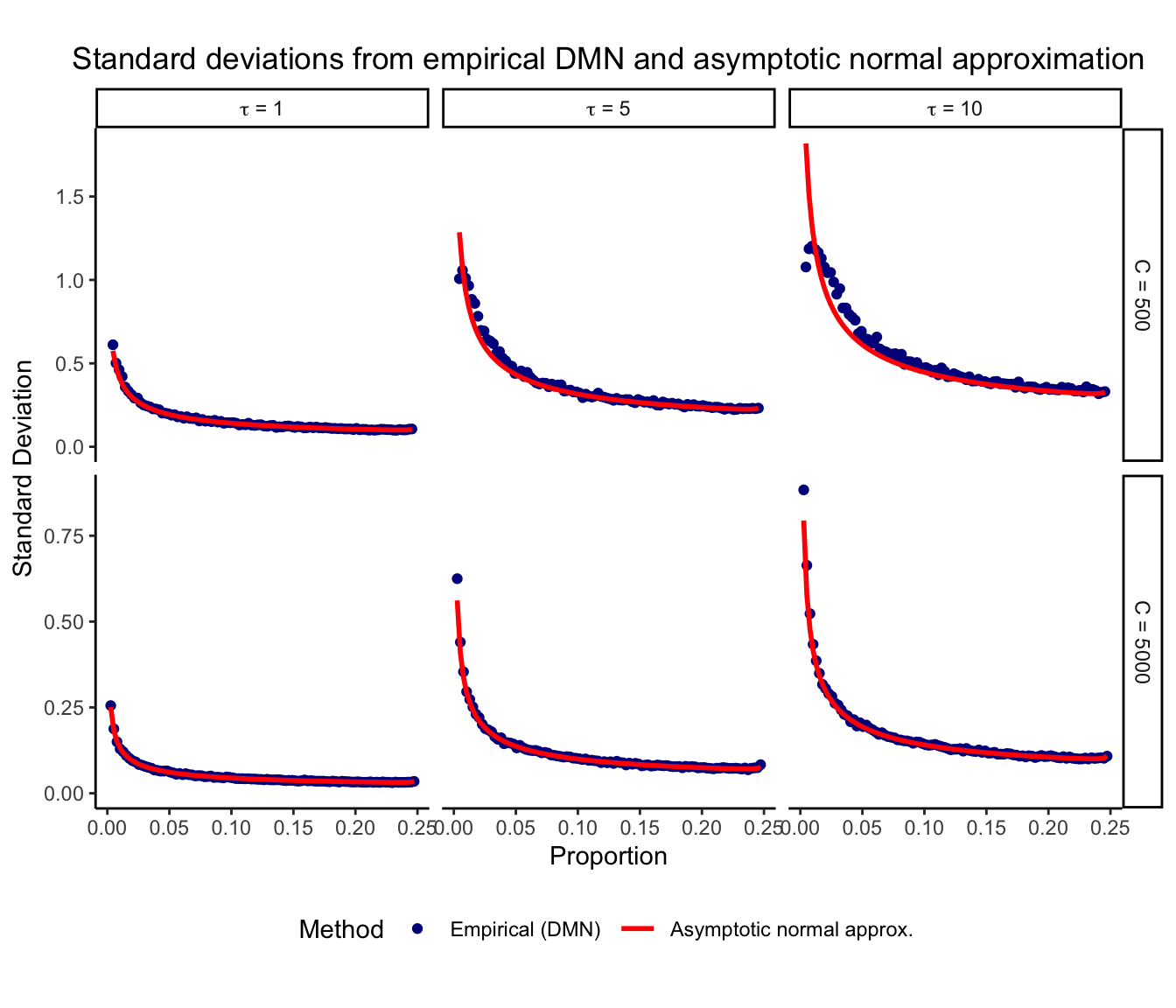
Interpretation

The asymptotic standard deviation shows good agreement with the empirical results even for small values of \(C\), when at least 2 counts are observed. In practice, it is often reasonable to assume a sufficient number of counts before a variable is included in an analysis. Importantly, with less than 2 counts the asymptotic theory gives a larger standard deviation than the emprical results (results not shown). Therefore, this approach is conservative and should not underestimate the true amount of variation. The asymptotic normal approximation is most accurate for large total counts \(C\), large proportions \(p\), and small overdispersion \(\tau\).

Consideration of overdispersion

Based on Equation (2), the variance of the CLR-transformed proportions is a linear function of \(\tau\). Importantly, downstream analysis of the CLR-transformed proportions with a precision-weighted linear (mixed) model or a variance stabilizing transform depends only on the relative variances. Since relative variances are invariant to the scale of \(\tau\), for these applications the value of \(\tau\) can be set to 1 instead of being estimated from the data.

For other applications, crumblr can estimate \(\tau\) from the data by using crumblr(counts, tau=NULL). This calls dmn.mle() to estimate the parameters of the DMN distribution and is substantially faster than alternatives.