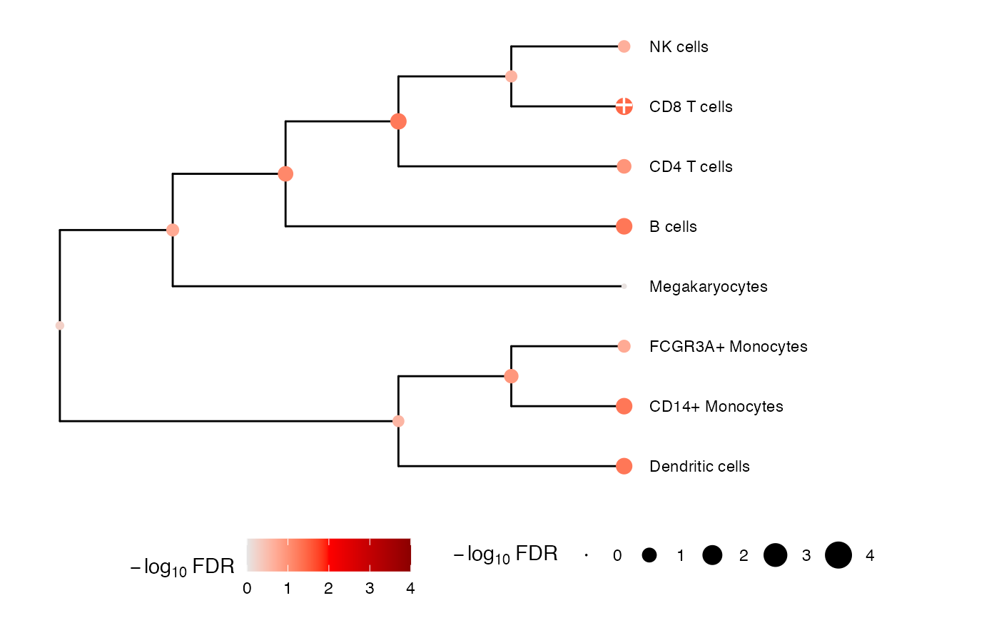
Perform multivariate testing along a hierarchy

Perform multivariate testing using mvTest() along the nodes of tree

Usage

treeTest(
  fit,
  obj,
  hc,
  coef,
  method = c("FE.empirical", "FE", "RE2C", "tstat", "sidak", "fisher"),
  shrink.cov = TRUE
)

Arguments

fit

MArrayLM object return by lmFit() or dream()

obj

EList object returned by voom()

hc

hierarchical clustering as an hclust object

coef

name of coefficient to be extracted

method

statistical method used to perform multivariate test. See details. 'FE' is a fixed effect test that models the covariance between coefficients. 'FE.empirical' use compute empirical p-values by sampling from the null distribution and fitting with a gamma. 'RE2C' is a random effect test of heterogeneity of the estimated coefficients that models the covariance between coefficients, and also incorporates a fixed effects test too. 'tstat' combines the t-statistics and models the covariance between coefficients. 'sidak' returns the smallest p-value and accounting for the number of tests. 'fisher' combines the p-value using Fisher's method assuming independent tests.

shrink.cov

shrink the covariance matrix between coefficients using the Schafer-Strimmer method

Details

See package remaCor for details about the remaCor::RE2C() test, and see remaCor::LS() for details about the fixed effect test. When only 1 feature is selected, the original t-statistic and p-value are returned.

See also

variancePartition::mvTest

Examples

library(variancePartition)

# Load cell counts, clustering and metadata
# from Kang, et al. (2018) https://doi.org/10.1038/nbt.4042
data(IFNCellCounts)

# Apply crumblr transformation
cobj <- crumblr(df_cellCounts)

# Use dream workflow to analyze each cell separately
fit <- dream(cobj, ~ StimStatus + ind, info)
fit <- eBayes(fit)

# Perform multivariate test across the hierarchy
res <- treeTest(fit, cobj, hcl, coef = "StimStatusstim")

# Plot hierarchy and testing results
plotTreeTest(res)


# Extract results for first 3 nodes
res[1:3, ]
#> # A tibble: 3 × 9
#>    node    beta     se  stat pvalue n_features lambda method          FDR
#>   <int>   <dbl>  <dbl> <dbl>  <dbl>      <dbl>  <dbl> <chr>         <dbl>
#> 1     1 -0.105  0.0348 -3.01 0.0137          1   0.01 FE.empirical 0.0513
#> 2     2 -0.105  0.0337 -3.12 0.0114          1   0.01 FE.empirical 0.0513
#> 3     3 -0.0784 0.0351 -2.23 0.0509          1   0.01 FE.empirical 0.109